
Last updated: June 11, 2026
In simple terms: xG assigns a probability between 0 and 1 to every shot, based on its historical likelihood of becoming a goal from that location, angle, and context. A value of 0.35 means that type of chance, from that location and angle, has been converted 35% of the time historically. It measures shot quality – not just whether the ball went in.
In the 72nd minute, a striker breaks through one-on-one. Clean sight of goal. He shoots – and misses. The crowd calls it a wasted chance. xG tells a different story: that attempt carried a 0.41 probability. The striker did everything right. The outcome was just variance.
The Expected Goals model provides that context. Built on machine learning trained against hundreds of thousands of historical shots, it strips away luck and exceptional goalkeeping to expose the underlying quality of a team’s attacking process. For the strategist, it doesn’t rewrite scorelines – it diagnoses whether a performance is sustainable.
While xG measures the quality of a shot, it cannot explain how that chance was created. High xG numbers are usually the result of a dominant tactical structure that controls space and possession. To see how elite teams build these structures, check out our master framework in Football Tactics: The 5 Phases of the Game.
This article dissects the mechanics of Expected Goals model, moving beyond the surface-level definitions to explore the specific variables – from defensive pressure to shot clarity – that define elite goal-scoring models.
See my full breakdown on how Build-Up Play structures generate high-xG chances
Key Takeaways
- xG doesn’t predict goals – it diagnoses process.
It tells you whether chances are repeatable, not whether a shot went in once. - Shot volume is noise without context.
Ten low-quality shots mean less than one well-structured cut-back inside the box. - Distance and angle matter more than instinct.
Most “great goals” are low-probability events – sustainable attacks live in boring zones. - Elite finishers don’t break xG – they bend it slightly.
Over time, even the best players regress toward probability. - Tactical structure creates xG, not individual brilliance.
Systems that generate cut-backs and central access will always win the numbers.
Table of Contents
The Mechanics: How xG Models Are Calculated
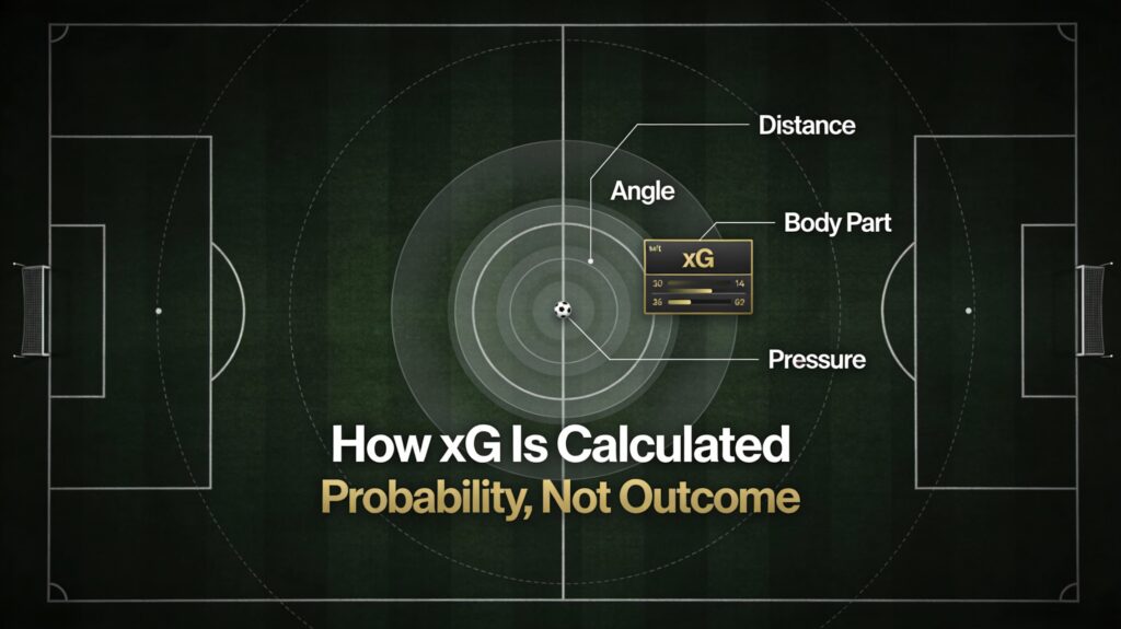
xG measures the quality of a single shot by assigning a probability between 0 and 1, based on how often that type of chance has been converted historically across hundreds of thousands of shots. If a specific type of chance has historically resulted in a goal 15 times out of 100, that shot is assigned an Expected Goals value of 0.15.
The calculation is derived from analyzing hundreds of thousands of shots from historical match data. Advanced models, such as those used by StatsBomb, utilize granular data points including the position of the goalkeeper and the pressure applied by defenders.
Basic models might look only at the location of the shot. However, a strategist must understand that location is only one factor. A header from the penalty spot has a significantly lower conversion rate than a shot with the stronger foot from the same position. Therefore, elite models layer multiple variables to refine the probability.
Strategist Note: xG is cumulative. A team that generates 2.50 xG in a match did not necessarily “miss” 2.5 goals; rather, the cumulative probability of their chances suggested they created enough quality to score approximately two to three times.
This is the foundational argument Chris Anderson and David Sally laid out in The Numbers Game: football is a low-scoring, noise-heavy sport, and metrics like xG exist precisely because single-match outcomes are unreliable evidence on their own.
Variables of Probability: Distance, Angle, and Context
To truly understand “What is xG,” we must isolate the specific variables that feed the algorithm. The variance in model accuracy often depends on how many of these variables are included.
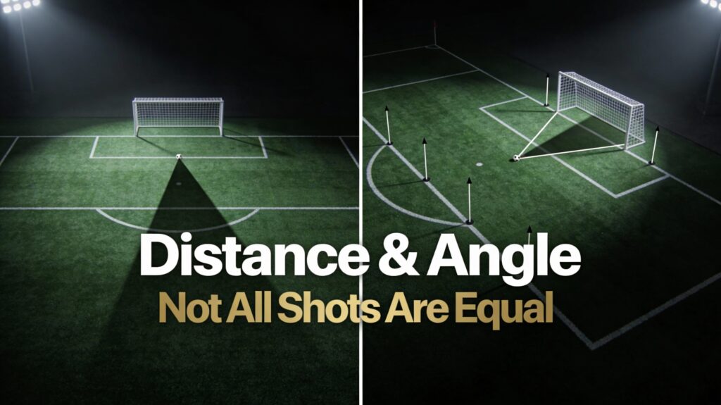
1. Distance to Goal
This is the most significant variable. The correlation is negative and non-linear; as distance increases, the probability of scoring drops precipitously. A shot from the edge of the six-yard box often carries an xG of >0.35, while a strike from 25 yards usually sits below 0.03.
2. Angle of the Shot
The width of the visible goalmouth decreases as the angle becomes more acute. A shot from the center of the box offers the maximum target area. As a player moves to the wide channels, the goalkeeper’s positioning can effectively block the entire goalface, reducing xG to near zero regardless of distance.
3. Body Part
Footedness and headers matter. Shots taken with a player’s strong foot generally have higher conversion rates than weak-footed shots. Headers, even from close range, have lower xG values than shots because of the difficulty in controlling the trajectory and velocity of the ball.
4. Type of Assist (The “Big Chance” Factor)

The context of the delivery is crucial. A “cut-back” pass from the byline – often seen in Pep Guardiola’s Final Third Mechanics – drastically increases xG because it often eliminates the goalkeeper or defenders from the equation. Conversely, a cross into a crowded box has a lower success rate due to defensive interference.
Interpreting Variance: Over performance vs. Sustainability
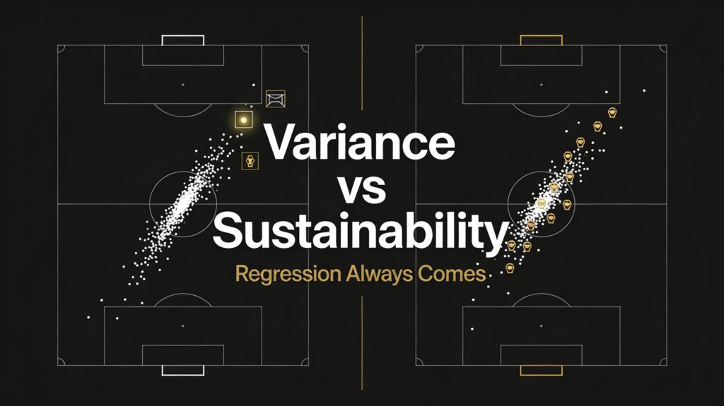
One of the most valuable applications of xG for a strategist is identifying variance. When a team or player significantly overperforms their expected scoring value (scoring more goals than the model predicts), it usually indicates one of two things:
- Elite Finishing: Players like Erling Haaland and Mohamed Salah have historically outperformed their xG over large sample sizes – Haaland’s 2024-25 season saw him score above his cumulative xG across all competitions, reflecting elite positioning in high-value zones rather than low-probability heroics. Their finishing technique exceeds the “average” player the model is calibrated against.
- Unsustainable “Hot” Streaks: For most players, a massive overperformance (e.g., scoring 10 goals from 4.0 Expected Goals) is a statistical anomaly that will likely regress to the mean over time.
Conversely, underperformance can signal bad luck or a lack of confidence, rather than a systemic tactical failure. If a team is generating high expected goals but not scoring, a manager may choose to persist with the tactic, trusting that the goals will eventually arrive as probability evens out.
Tactical Table: High xG vs. Low xG Scenarios
The following table categorizes common match scenarios and their approximate xG values to provide a baseline for analysis.
How Much xG Is a Penalty?
Penalties are assigned 0.76 xG in most major models, including Opta and StatsBomb. This makes them the highest-probability standard situation in football – a static ball, maximum distance from defenders, only the goalkeeper to beat. The roughly 24% non-conversion rate accounts for saves, posts, and wayward strikes across the historical dataset.
| Scenario | Approx. xG | Tactical Context |
| Penalty Kick | 0.76 – 0.79 | The highest probability standard situation in football. A static ball with only the keeper to beat. |
| Tap-in (Central) | 0.50 – 0.65 | Usually the result of a square pass or rebound inside the six-yard box. |
| 1v1 vs. Keeper | 0.30 – 0.50 | Dependent on the time the attacker has and the keeper’s starting position. |
| Cut-back Shot | 0.25 – 0.40 | High value due to the keeper often being caught moving laterally. |
| Header (Corner) | 0.08 – 0.12 | Low probability due to defensive crowding and aerial difficulty. |
| Long Shot (25y+) | 0.02 – 0.04 | “Low percentage” plays often forced by effective Low Block defenses. |
See Article #2 regarding Low Block Defense strategies to force low-xG shots
Limitations of the Model
While Expected Goals model is a powerful diagnostic tool, it is not infallible. A rigid adherence to the metric without video analysis can lead to false conclusions.
- Defensive Pressure: Basic Expected Goals models may not fully account for a defender blocking the shooting lane. A shot taken with three defenders in front is far harder than one taken in open space, even if the location is identical.
- Goalkeeper Impact: Expected Goals model measures the shot quality, not the save quality. Post-Shot xG (PSxG) is a variant metric used to evaluate goalkeepers, analyzing the shot’s trajectory after it leaves the boot.
- Game State: Teams chasing a game may accumulate “empty” xG by taking many low-quality shots, inflating their total without genuinely threatening the defense.
Understanding these nuances distinguishes elite recruitment departments from those simply following spreadsheets.
Pulling It All Together
Expected Goals should be viewed as a compass, not a scoreboard. It tells us the direction of travel – whether a team’s attacking process is healthy or reliant on unsustainable luck. For the tactical analyst, “What is xG?” is less about the number itself and more about the story it tells regarding spatial control and decision-making in the final third.
When we analyzedXabi Alonso’s Leverkusen Blueprint, we saw how tactical structures are designed specifically to maximize high-xG cut-backs while minimizing low-value long shots. Understanding Expected Goals Model is the first step in seeing the game through the lens of probability rather than just emotion.
What do you think?
Which metric do you find most useful in practice – standard xG, Post-Shot xG, or xA – and do you think the model gives a fair picture of a striker’s true quality?
Related Tactical Breakdowns

Expected Threat (xT) Explained]
Why it connects: xT measures the value of ball movement before the shot that xG evaluates – the two metrics map the full picture of how attacks build from progression to finish.

Why it connects: PSxG is the goalkeeper-evaluation layer built on top of xG – once you understand the base model, PSxG shows what shot-stopping above the expected baseline actually looks like.
Why it connects: PPDA measures how aggressively a team prevents the opponent from creating xG – understanding both metrics maps the full defensive-to-offensive data chain.
Don’t just watch football. Understand it.
Join KharaSportsDaily for occasional deep tactical insights most fans miss.
Frequently Asked Questions (FAQs)
Does xG account for the skill of the striker?
Generally, no. Standard xG models are based on the average conversion rate of thousands of players. This is why elite finishers consistently score slightly above their Expected Goals.
What is a “good” xG for a single match?
In top-tier leagues, a total team xG of 2.0+ usually indicates a dominant attacking performance. Anything below 0.8 suggests significant issues in chance creation.
Can a team win with a lower xG than their opponent?
Absolutely. Football is a low-scoring sport sensitive to high variance. A team can lose the “Expected Goals battle” but win the match through a moment of brilliance or a defensive error. However, consistently losing the xG battle usually leads to poor results over a season.
How does xG relate to xA (Expected Assists)?
xA assigns the Expected Goals value of the resulting shot to the player who made the final pass. It measures creativity and playmaking irrespective of whether the striker finishes the chance.
What is xG in football?
xG (Expected Goals) is a statistical measure assigning a probability between 0 and 1 to every shot based on its likelihood of becoming a goal, calculated using shot location, angle, assist type, and body part.
How is xG calculated?
xG is calculated using machine learning models trained on historical shot data, weighing variables including distance from goal, shot angle, body part used, assist type, and defensive pressure.
What is a good xG in football?
A match xG of 2.0+ typically indicates dominant chance creation. Individual shots range from 0.02 (long-range efforts) to 0.76 (penalties).